Project in R – Female Life Expectancy Project

Load the packages

library(tidyverse)
library(gghighlight)

Data Sources

Please download the data in CSV format from https://data.worldbank.org/indicator/SP.DYN.LE00.FE.IN
- Then unzip the .zip file and rename the unzipped folder as Original Data.
Indicator_code: SP.DYN.LE00.FE.IN
Data last updated date: 10/24/2024

Life expectancy at birth indicates the number of years a newborn infant would live if prevailing patterns of mortality at the time of its birth were to stay the same throughout its life.

Female Life Expectancy Data Source:

United Nations Population Division. World Population Prospects: 2022 Revision;
Statistical databases and publications from national statistical offices;
Eurostat: Demographic Statistics.

Three Datasets in the Original Data Folder

Dataset 1: API_SP.DYN.LE00.FE.IN_DS2_en_csv_v2_11541.csv

The variables are: Country Name, Country Code, Indicator Name, Indicator Code, 1960 – 2022.

Dataset 2: Metadata_Country_API_SP.DYN.LE00.FE.IN_DS2_en_csv_v2_11541.csv

Country Information Data, the variable are Country Code, Region, IncomeGroup, SpecialNotes, TableName.

Dataset 3: Metadata_Indicator_API_SP.DYN.LE00.FE.IN_DS2_en_csv_v2_11541.csv

This data will NOT be used in this project.

Data Cleaning

Import Data and check missing values

LE <- read_csv("Original Data/API_SP.DYN.LE00.FE.IN_DS2_en_csv_v2_11541.csv", skip = 4)
LE %>%
    dplyr::select(everything()) %>%
    summarize_all(~sum(is.na(.))) %>%
    print(width = Inf)  # show all the columns
#> # A tibble: 1 × 69
#>   `Country Name` `Country Code` `Indicator Name` `Indicator Code` `1960` `1961`
#>            <int>          <int>            <int>            <int>  <int>  <int>
#> 1              0              0                0                0     14     13
#>   `1962` `1963` `1964` `1965` `1966` `1967` `1968` `1969` `1970` `1971` `1972`
#>    <int>  <int>  <int>  <int>  <int>  <int>  <int>  <int>  <int>  <int>  <int>
#> 1     13     14     14     14     13     13     13     13     13     13     13
#>   `1973` `1974` `1975` `1976` `1977` `1978` `1979` `1980` `1981` `1982` `1983`
#>    <int>  <int>  <int>  <int>  <int>  <int>  <int>  <int>  <int>  <int>  <int>
#> 1     12     13     13     13     13     11     12     11     11     11     11
#>   `1984` `1985` `1986` `1987` `1988` `1989` `1990` `1991` `1992` `1993` `1994`
#>    <int>  <int>  <int>  <int>  <int>  <int>  <int>  <int>  <int>  <int>  <int>
#> 1     11     11     10     10     10     10      8      9      9      9      8
#>   `1995` `1996` `1997` `1998` `1999` `2000` `2001` `2002` `2003` `2004` `2005`
#>    <int>  <int>  <int>  <int>  <int>  <int>  <int>  <int>  <int>  <int>  <int>
#> 1      7      8      8      8      8      7      8      8      8      8      7
#>   `2006` `2007` `2008` `2009` `2010` `2011` `2012` `2013` `2014` `2015` `2016`
#>    <int>  <int>  <int>  <int>  <int>  <int>  <int>  <int>  <int>  <int>  <int>
#> 1      8      8      8      8      8      8      8      8      8      8      8
#>   `2017` `2018` `2019` `2020` `2021` `2022` `2023` ...69
#>    <int>  <int>  <int>  <int>  <int>  <int>  <int> <int>
#> 1      8      9      9      9      8      9    266   266

country <- read_csv("Original Data/Metadata_Country_API_SP.DYN.LE00.FE.IN_DS2_en_csv_v2_11541.csv")

country %>%
    dplyr::select(everything()) %>%
    summarize_all(~sum(is.na(.))) %>%
    print(width = Inf)  # show all the columns
#> # A tibble: 1 × 6
#>   `Country Code` Region IncomeGroup SpecialNotes TableName  ...6
#>            <int>  <int>       <int>        <int>     <int> <int>
#> 1              0     48          49          138         0   265

In LE, We should remove columns 2023 and ...69 since they are empty columns.
In country, we should remove column ...6.

LE <- LE %>%
    select(-`2023`, -...69)
country <- country %>%
    select(-...6)

Check the distinct values

LE %>%
    dplyr::select(everything()) %>%
    summarize_all(~n_distinct(.)) %>%
    print(width = Inf)
#> # A tibble: 1 × 67
#>   `Country Name` `Country Code` `Indicator Name` `Indicator Code` `1960` `1961`
#>            <int>          <int>            <int>            <int>  <int>  <int>
#> 1            266            266                1                1    247    248
#>   `1962` `1963` `1964` `1965` `1966` `1967` `1968` `1969` `1970` `1971` `1972`
#>    <int>  <int>  <int>  <int>  <int>  <int>  <int>  <int>  <int>  <int>  <int>
#> 1    249    247    244    249    248    251    249    250    249    251    248
#>   `1973` `1974` `1975` `1976` `1977` `1978` `1979` `1980` `1981` `1982` `1983`
#>    <int>  <int>  <int>  <int>  <int>  <int>  <int>  <int>  <int>  <int>  <int>
#> 1    250    249    248    249    246    252    249    252    247    251    251
#>   `1984` `1985` `1986` `1987` `1988` `1989` `1990` `1991` `1992` `1993` `1994`
#>    <int>  <int>  <int>  <int>  <int>  <int>  <int>  <int>  <int>  <int>  <int>
#> 1    252    249    252    250    250    251    253    250    253    250    254
#>   `1995` `1996` `1997` `1998` `1999` `2000` `2001` `2002` `2003` `2004` `2005`
#>    <int>  <int>  <int>  <int>  <int>  <int>  <int>  <int>  <int>  <int>  <int>
#> 1    254    251    250    250    247    248    245    248    243    243    247
#>   `2006` `2007` `2008` `2009` `2010` `2011` `2012` `2013` `2014` `2015` `2016`
#>    <int>  <int>  <int>  <int>  <int>  <int>  <int>  <int>  <int>  <int>  <int>
#> 1    248    246    242    245    244    240    244    245    245    245    245
#>   `2017` `2018` `2019` `2020` `2021` `2022`
#>    <int>  <int>  <int>  <int>  <int>  <int>
#> 1    244    247    244    246    247    247

country %>%
    dplyr::select(everything()) %>%
    summarize_all(~n_distinct(.)) %>%
    print(width = Inf)
#> # A tibble: 1 × 5
#>   `Country Code` Region IncomeGroup SpecialNotes TableName
#>            <int>  <int>       <int>        <int>     <int>
#> 1            265      8           5          114       265

We delete the Indicator Name and Indicator Code in LE
We delete the SpecialNotes and TableName in country

LE <- LE %>%
    dplyr::select(-`Indicator Name`, -`Indicator Code`) %>%
    filter(complete.cases(.))  # Remove the observations with missing values

country <- country %>%
    dplyr::select(-SpecialNotes, -TableName) %>%
    filter(complete.cases(.))

Tidy and Join

LE <- LE %>%
    pivot_longer(`1960`:`2022`, names_to = "Year", values_to = "life_expectancy") %>%
    rename(CountryName = `Country Name`, CountryCode = `Country Code`)

country <- country %>%
    rename(CountryCode = `Country Code`)


LE_ctry <- LE %>%
    inner_join(country, by = "CountryCode")

dim(LE_ctry)
#> [1] 12726     6

There are 12726 observations and 6 columns.

Data Visualization

LE_ctry %>%
    group_by(CountryName) %>%
    dplyr::summarize(country_mean = mean(life_expectancy)) %>%
    ggplot(aes(x = CountryName, y = country_mean)) + geom_col()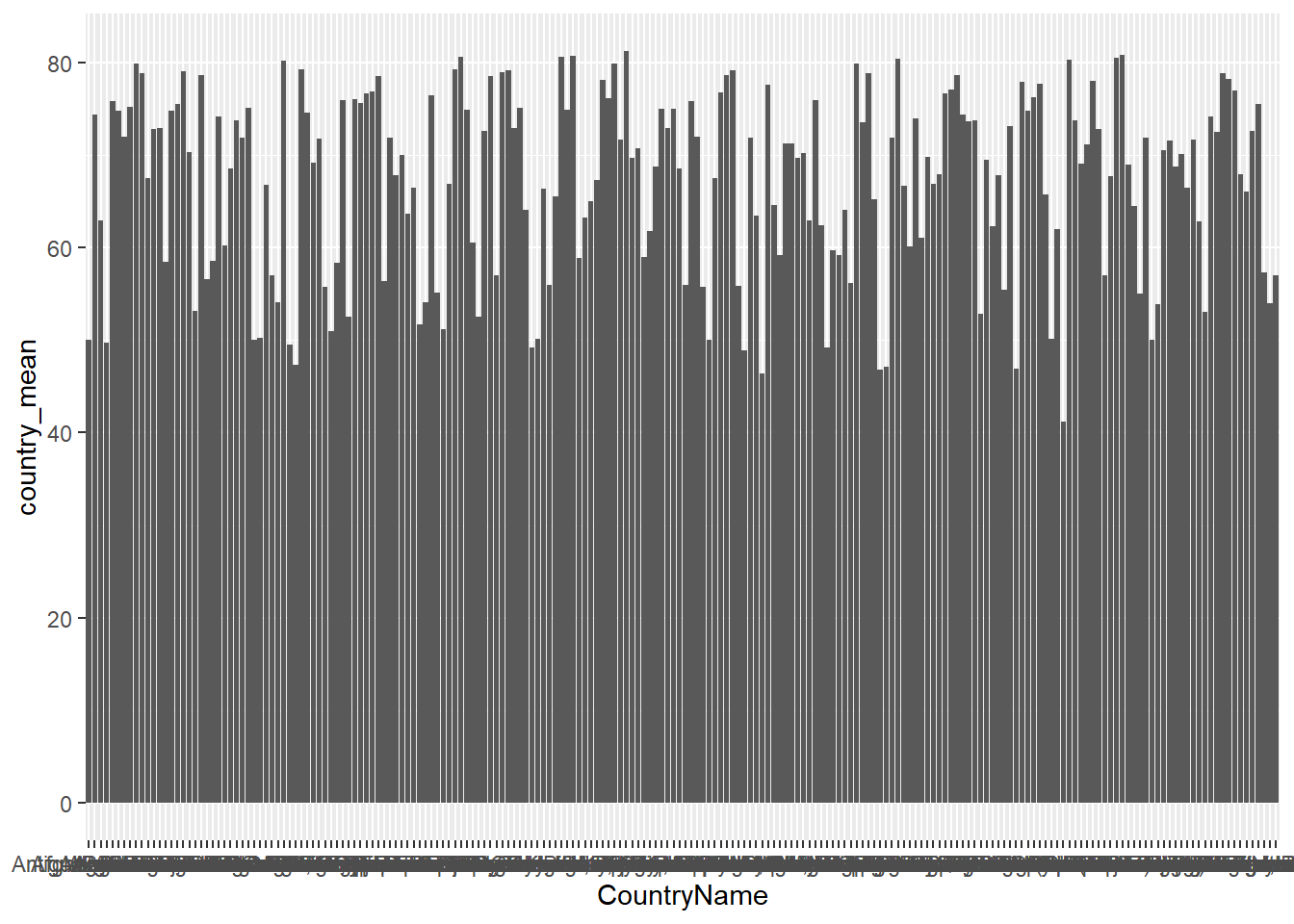

Top 10 LE

LE_ctry %>%
    group_by(CountryName) %>%
    dplyr::summarize(country_mean = mean(life_expectancy)) %>%
    arrange(desc(country_mean)) %>%
    top_n(10) %>%
    mutate(CountryName = fct_inorder(CountryName)) %>%
    ggplot(aes(x = CountryName, y = country_mean)) + geom_col() + labs(x = "Country Name",
    y = "Average Life Expectancy") + theme_minimal() + theme(axis.text.x = element_text(angle = 45))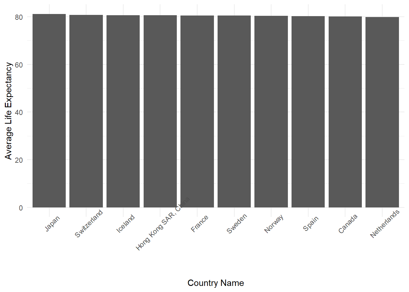

Female life expectancy by year – highlight the top 3


LE_ctry <- LE_ctry %>%
    group_by(CountryName) %>%
    mutate(country_avg = mean(life_expectancy))

LE_ctry %>%
    ggplot(aes(x = as.numeric(Year), y = life_expectancy, color = CountryName)) +
    geom_line() + gghighlight(country_avg > 80.65)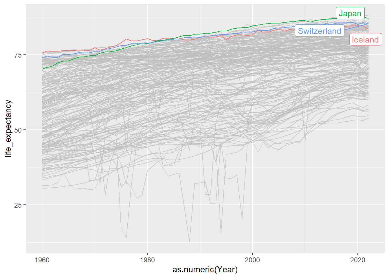

Summary of result:

Japan, Iceland, Switzerland are the top 3 countries with high female life expectancy on average.

Life Expectancy vs Income Group

LE_ctry <- LE_ctry %>%
    mutate(IncomeGroup = factor(IncomeGroup, levels = c("High income", "Upper middle income",
        "Lower middle income", "Low income")))


LE_ctry %>%
    ggplot(aes(x = as.numeric(Year), y = life_expectancy, group = CountryName, color = IncomeGroup)) +
    geom_line() + theme_minimal() + labs(title = "Female life expectancy for different income groups",
    x = "Year", y = "Life Expectancy", color = "Income Group")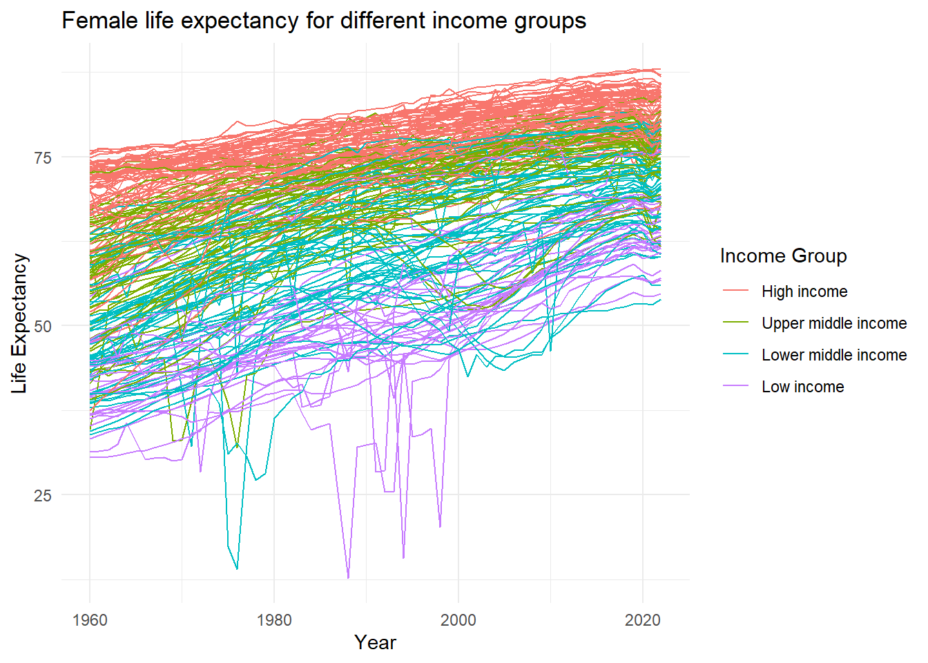

Conclusion:

High income countries generally have higher female life expectancy.
Low income countries have lower female life expenctancy.