(A <- matrix(1:4, nrow = 2))
#>      [,1] [,2]
#> [1,]    1    3
#> [2,]    2    4
(B <- matrix(c(0, 6, 5, 7), nrow = 2))
#>      [,1] [,2]
#> [1,]    0    5
#> [2,] 6 7STAT 385 Lab 5 Vectorization Help Document
Why Vectorization?
- Avoid using for loops in R when possible.
- Use vectorization whenever you can.
Kronecker Product
In mathematics, the Kronecker product, sometimes denoted by \(\bigotimes\), is an operation on two matrices of arbitrary size resulting a block matrix. It is a specialization of the tensor product (which is denoted by the same symbol) from vectors to matrices and gives the matrix of the tensor product linear map with respect to a standard choice of basis. The Kronecker product is to be distinguished from the usual matrix multiplication, which is an entirely different operation. The Kronecker product is also sometimes called matrix direct product.
- You can find more information about Kronecker Product on Wikipedia https://en.wikipedia.org/wiki/Kronecker_product.
Mathemetical Definition of Kronecker Product
If \(\mathbf{A}\) is an \(m \times n\) matrix and \(\mathbf{B}\) is a \(p \times q\) matrix, then the Kronecker product \(\mathbf{A}\bigotimes \mathbf{B}\) is the \(pm \times qn\) block matrix:
\[\mathbf{A}\bigotimes \mathbf{B} = \begin{bmatrix} a_{11}\mathbf{B}\quad \cdots \quad a_{1n}\mathbf{B}\\ \vdots\quad \ddots\quad \vdots\\ a_{m1}\mathbf{B}\quad \cdots \quad a_{mn}\mathbf{B} \end{bmatrix},\]
more explicitly,
\[\mathbf{A}\bigotimes \mathbf{B} =\left[\begin{array}{cccccccccc} a_{11}b_{11}& a_{11}b_{12} & \cdots & a_{11}b_{1q}& \cdots& \cdots& a_{1n}b_{11}& a_{1n}b_{12} & \cdots & a_{1n}b_{1q} \\ a_{11}b_{21}& a_{11}b_{22} & \cdots & a_{11}b_{2q}& \cdots& \cdots& a_{1n}b_{21}& a_{1n}b_{22} & \cdots & a_{1n}b_{2q} \\ \vdots& \vdots& \ddots& \vdots & & & \vdots& \vdots& \ddots& \vdots \\ a_{11}b_{p1}& a_{11}b_{p2} & \cdots & a_{11}b_{pq}& \cdots& \cdots& a_{1n}b_{p1}& a_{1n}b_{p2} & \cdots & a_{1n}b_{pq} \\ \vdots& \vdots& & \vdots & \ddots& & \vdots & \vdots& & \vdots \\ \vdots& \vdots& & \vdots & &\ddots & \vdots & \vdots& & \vdots \\ a_{m1}b_{11}& a_{m1}b_{12} & \cdots & a_{m1}b_{1q}& \cdots& \cdots& a_{mn}b_{11}& a_{mn}b_{12} & \cdots & a_{mn}b_{1q} \\ a_{m1}b_{21}& a_{m1}b_{22} & \cdots & a_{m1}b_{2q}& \cdots& \cdots& a_{mn}b_{21}& a_{mn}b_{22} & \cdots & a_{mn}b_{2q} \\ \vdots& \vdots& \ddots& \vdots & & & \vdots& \vdots& \ddots& \vdots \\ a_{m1}b_{p1}& a_{m1}b_{p2} & \cdots & a_{m1}b_{pq}& \cdots& \cdots& a_{mn}b_{p1}& a_{mn}b_{p2} & \cdots & a_{mn}b_{pq} \end{array}\right],\]
Kronecker Product Example
\[A = \begin{bmatrix} 1 \quad 3 \\ 2 \quad 4 \end{bmatrix}\]
\[B = \begin{bmatrix} 0 \quad 5 \\ 6 \quad 7 \end{bmatrix}\]
Then
\[\mathbf{A}\bigotimes \mathbf{B} = \left[\begin{array}{cccc} 1\times 0 & 1\times 5 & 3\times 0 & 3\times 5\\ 1\times 6 & 1\times 7 & 3\times 6 & 3\times 7\\ 2\times 0 & 2\times 5 & 4\times 0 & 4\times 5\\ 2\times 6 & 2\times 7 & 4\times 6 & 4\times 7 \end{array}\right] = \left[\begin{array}{cccc} 0 & 5 & 0 & 15\\ 6 & 7 & 18 & 21\\ 0 & 10 & 0 & 20\\ 12 & 14 & 24 & 28 \end{array}\right].\]
Calculate Kronecker Product in R
Let \(A\) and \(B\) be \(2 \times 2\) matrices as follows:
Method I: The kronecker() Function
A
#>      [,1] [,2]
#> [1,]    1    3
#> [2,]    2    4
B
#>      [,1] [,2]
#> [1,]    0    5
#> [2,]    6    7
kronecker(A, B)
#>      [,1] [,2] [,3] [,4]
#> [1,]    0    5    0   15
#> [2,]    6    7   18   21
#> [3,]    0   10    0   20
#> [4,]   12   14   24   28
Method II: For Loop
\[\mathbf{A}\bigotimes \mathbf{B} = \left[\begin{array}{cccc} 1\times 0 & 1\times 5 & 3\times 0 & 3\times 5\\ 1\times 6 & 1\times 7 & 3\times 6 & 3\times 7\\ 2\times 0 & 2\times 5 & 4\times 0 & 4\times 5\\ 2\times 6 & 2\times 7 & 4\times 6 & 4\times 7 \end{array}\right] = \left[\begin{array}{cccc} 0 & 5 & 0 & 15\\ 6 & 7 & 18 & 21\\ 0 & 10 & 0 & 20\\ 12 & 14 & 24 & 28 \end{array}\right].\] Locations:
forloop_kronecker <- function(A, B){
  Res = matrix(NA, nrow = 2*2, ncol = 2*2)
  k = 0
  l = 0

  for (j in 1:2){
    k = 0
    for (i in 1:2){
      Res[(k+1):(k+2), (l+1):(l+2)] <- A[i, j] * B
      k = k + 2
    }
    l = l + 2
  }
  Res
}

forloop_kronecker(A, B)
#>      [,1] [,2] [,3] [,4]
#> [1,]    0    5    0   15
#> [2,]    6    7   18   21
#> [3,]    0   10    0   20
#> [4,]   12   14   24   28
Method III: Vectorization [Recommended]
Objective
Deal with A
Recall
rep(1:2, each = 2)
#> [1] 1 1 2 2
A
#> [,1] [,2]
#> [1,] 1 3
#> [2,] 2 4
A[rep(1:2, each = 2), rep(1:2, each = 2)]
#> [,1] [,2] [,3] [,4]
#> [1,] 1 1 3 3
#> [2,] 1 1 3 3
#> [3,] 2 2 4 4
#> [4,] 2 2 4 4Deal with B
Recall
rep(1:2, times = 2)
#> [1] 1 2 1 2
B
#> [,1] [,2]
#> [1,] 0 5
#> [2,] 6 7
B[rep(1:2, times = 2), rep(1:2, times = 2)]
#> [,1] [,2] [,3] [,4]
#> [1,] 0 5 0 5
#> [2,] 6 7 6 7
#> [3,] 0 5 0 5
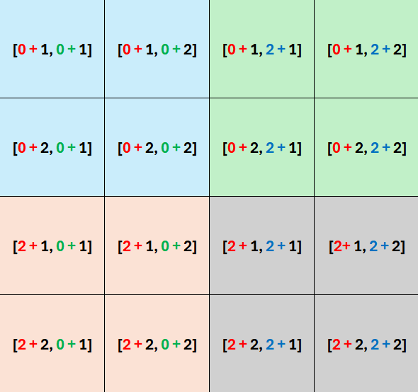
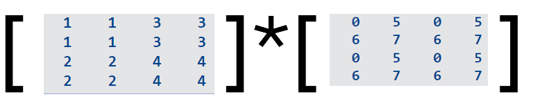
#> [4,] 6 7 6 7Put Everything Together
repeated_A <- A[rep(1:2, each = 2), rep(1:2, each = 2)]
repeated_B <- B[rep(1:2, times = 2), rep(1:2, times = 2)]
repeated_A * repeated_B
#>      [,1] [,2] [,3] [,4]
#> [1,]    0    5    0   15
#> [2,]    6    7   18   21
#> [3,]    0   10    0   20
#> [4,]   12   14   24   28
Wrap the Calculation into a Function (for \(2 \times 2\) matrices)
vectorization_kronecker <- function(A, B){
  repeated_A <- A[rep(1:2, each = 2), rep(1:2, each = 2)]
  repeated_B <- B[rep(1:2, times = 2), rep(1:2, times = 2)]
  return(repeated_A * repeated_B)
}

vectorization_kronecker(A, B)
#>      [,1] [,2] [,3] [,4]
#> [1,]    0    5    0   15
#> [2,]    6    7   18   21
#> [3,]    0   10    0   20
#> [4,]   12   14   24   28
Compare the CPU Times that Expressions Used
microbenchmark::microbenchmark(
  vectorization_kronecker(A,B),
  kronecker(A, B),
  forloop_kronecker(A, B),
  times=10000L
)
#> Unit: microseconds
#>                           expr  min   lq     mean median uq    max neval
#>  vectorization_kronecker(A, B)  2.8  3.4  6.40591    5.9  7 5157.1 10000
#>                kronecker(A, B) 23.2 24.9 44.00815   50.5 54 2498.2 10000
#>        forloop_kronecker(A, B)  4.7  5.4  9.86099   10.4 12 2148.8 10000
What if A and B are not \(2 \times 2\) matrices?
With the assistance of this instructional document, please proceed with Lab 5.
In Lab 5, you will update the forloop_kronecker() and vectorization_kronecker() functions to make them suitable for calculating matrices A and B with arbitrary dimensions. And find result similar to the following.
A1 <- matrix(1:16, nrow = 4, ncol = 4)
B1 <- matrix(1:20, nrow = 4, ncol = 5)

A2 <- matrix(1:40, nrow = 5, ncol = 8)
B2 <- matrix(1:50, nrow = 10, ncol = 5)- Compare the CPU Times that Expressions Used for
A1andB1
# A1 and B1
microbenchmark::microbenchmark(
  vectorization_kronecker(A1,B1),
  kronecker(A1, B1),
  forloop_kronecker(A1, B1),
  times=10000L
)
#> Unit: microseconds
#>                             expr  min   lq     mean median   uq     max neval
#>  vectorization_kronecker(A1, B1)  7.9  9.3 13.88071    9.9 16.8  4753.6 10000
#>                kronecker(A1, B1) 24.7 27.9 43.97730   29.8 58.7  3307.9 10000
#> forloop_kronecker(A1, B1) 36.7 41.2 61.62278 43.3 76.1 18219.7 10000- Compare the CPU Times that Expressions Used for
A2andB2
# A2 and B2

microbenchmark::microbenchmark(
  vectorization_kronecker(A2,B2),
  kronecker(A2, B2),
  forloop_kronecker(A2, B2),
  times=10000L
)
#> Unit: microseconds
#>                             expr  min    lq      mean median    uq    max neval
#>  vectorization_kronecker(A2, B2) 14.5  18.9  31.77746  24.90  38.4 6298.2 10000
#>                kronecker(A2, B2) 29.3  45.1  82.59700  64.45 102.9 6145.0 10000
#>        forloop_kronecker(A2, B2) 79.8 100.3 164.87652 120.70 206.4 9142.7 10000