Lab 4
Question 1
Estimate the value of \(\pi\) by using probability simulation.
- [20 pts] Use
set.seed(10). Please generate a set of \(n = 10,000\) random points \((x_i, y_i)\), within the square defined by the Cartesian coordinates \([-1, 1] \times [-1, 1]\) . For each point, check if it lies inside a circle with radius 1 centered at the origin. Store the \(x\)- and \(y\)-coordinates of points inside the circle in vectorsin_circle_xandin_circle_y, respectively. Similarly, store the coordinates of points outside the circle in vectorsout_circle_xandout_circle_y.
[Hints:
- You may use
runif()for taking the random points. Use?runif()if needed. - You may use if…else statement and for loop for this question.]
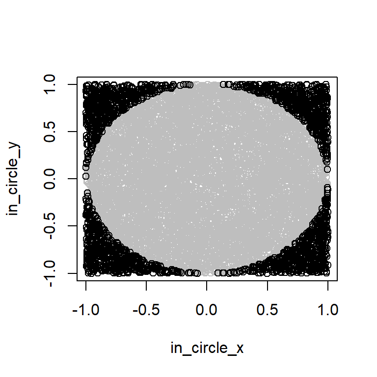
- [10 pts] Draw the simulation points using
plot()andpoints()by coloring the in-circle points blue and out-circle points orange.
The plot should be resemble something like this with the required color.
[Hints:
- Use
plot()to draw points. - Use
points()to add points to the plot above. - Use
col = "blue"andcol = "orange"for the colors. ]
- [10 pts] Complete the blanks below.
There are two different ways to calculate the probability of points fall in the circle.
: The probability \(= \frac{\text{Number of points in the in\_circle\_x (or in\_circle\_y)}}{\text{Total number of points in x (or y)}}\).
### Use R code to find the probability using Method I: The probability \(=\frac{\text{Area of circle}}{\text{Area of square}} = \frac{ }{ }\). [Hint: The radius of the circle is 1, and the side-length of the square is \(1-(-1) = 2\). ]
- [5 pts] Based on the result in (c), estimate the value of \(\pi\).
Question 2 Create a function to add an additional row to the ANOVA table output.
Below are the codes you’ll learn in STAT 425. But we will set aside the interpretation of the codes and results for now. In this question, we’ll only focus on adding an additional row to the ANOVA Table output.
To be specific, in this question, we will work on defining a new function called anova_tab(). So that, compare to the default anova() below, anova_tab() can have the additional row needed. Please complete this task by addressing the following subquestions.
PG.mod <- lm(weight ~ group, data = PlantGrowth) # PG.mod is an lm objectanova() output for PG.mod
PG.mod_aov <- anova(PG.mod)
PG.mod_aov
#> Analysis of Variance Table
#>
#> Response: weight
#>           Df  Sum Sq Mean Sq F value  Pr(>F)
#> group      2  3.7663  1.8832  4.8461 0.01591 *
#> Residuals 27 10.4921  0.3886
#> ---
#> Signif. codes:  0 '***' 0.001 '**' 0.01 '*' 0.05 '.' 0.1 ' ' 1
anova_tab() output for PG.mod
anova_tab(PG.mod)
#> Analysis of Variance Table
#>
#> Response: weight
#>           Df  Sum Sq Mean Sq F value  Pr(>F)
#> group      2  3.7663  1.8832  4.8461 0.01591 *
#> Residuals 27 10.4921  0.3886
#> Total     29 14.2584
#> ---
#> Signif. codes: 0 '***' 0.001 '**' 0.01 '*' 0.05 '.' 0.1 ' ' 1- [5 pts] Check if
PG.mod_aovis a list. Then check ifPG.mod_aovis a data frame. If the object is a data frame, determine its dimension (i.e., the number of rows and columns).
- [10 pts] Add the third row to
PG.mod_aovwhere
- the first element is the sum of the two “DF” values,
- the second element is the sum of the two “Sum Sq” values,
- the remaining three elements are NA,
- and name this new row “Total”.
- [10 pts] Another regression example using
mtcars,
mt.mod <- lm(mpg ~ hp + wt, data = mtcars) # mt.mod is an lm object
mt.mod_aov <- anova(mt.mod)
mt.mod_aov
#> Analysis of Variance Table
#>
#> Response: mpg
#>           Df Sum Sq Mean Sq F value    Pr(>F)
#> hp         1 678.37  678.37 100.862 5.987e-11 ***
#> wt         1 252.63  252.63  37.561 1.120e-06 ***
#> Residuals 29 195.05    6.73
#> ---
#> Signif. codes:  0 '***' 0.001 '**' 0.01 '*' 0.05 '.' 0.1 ' ' 1
Add a fourth row to mt.mod_aov where
- the first element is the sum of the three “DF” values,
- the second element is the sum of the three “Sum Sq” values,
- the remaining three elements are NA,
- and name this new row “Total”.
[Hint: To make the code more generalizable, you may use sum(mt.mod_aov[1:3, 1]), instead of mt.mod_aov[1, 1] + mt.mod_aov[2, 1] + mt.mod_aov[3, 1].]
- [10 pts] Part (b) and (c) provide concrete examples. Please create a function called
anova_tab()that takes anylmobject (such asPG.mod,mt.modin this question) as input and displays the ANOVA summary table, including the additional “Total” row. Then useanova_tab(PG.mod)andanova_tab(mt.mod)to test the function. Then useanova_tab(att.mod)below to test theanova_tab()function.
att.mod <- lm(rating ~ complaints + privileges + learning + raises, data = attitude)