Data Transformation with Pivot, Separate, Unite, and Join

Data Science Workflow

Workflow in data science, with Tidyverse – https://oliviergimenez.github.io/intro_tidyverse/#1

Tidy Data

Happy families are all alike; every unhappy family is unhappy in its own way. — Leo Tolstoy

Tidy datasets are all alike, but every messy dataset is messy in its own way. — Hadley Wickham, author of R for Data Science

• Tidy data is data where:
  • Every column is variables.
  • Every row is an observation.
  • Every cell is a single value.

library(tidyverse)
table1
#> # A tibble: 6 × 4
#>   country      year  cases population
#>   <chr>       <dbl>  <dbl>      <dbl>
#> 1 Afghanistan  1999    745   19987071
#> 2 Afghanistan  2000   2666   20595360
#> 3 Brazil       1999  37737  172006362
#> 4 Brazil       2000  80488  174504898
#> 5 China        1999 212258 1272915272
#> 6 China        2000 213766 1280428583
table2
#> # A tibble: 12 × 4
#>    country      year type            count
#>    <chr>       <dbl> <chr>           <dbl>
#>  1 Afghanistan  1999 cases             745
#>  2 Afghanistan  1999 population   19987071
#>  3 Afghanistan  2000 cases            2666
#>  4 Afghanistan  2000 population   20595360
#>  5 Brazil       1999 cases           37737
#>  6 Brazil       1999 population  172006362
#>  7 Brazil       2000 cases           80488
#>  8 Brazil       2000 population  174504898
#>  9 China        1999 cases          212258
#> 10 China        1999 population 1272915272
#> 11 China        2000 cases          213766
#> 12 China        2000 population 1280428583
table3
#> # A tibble: 6 × 3
#>   country      year rate             
#>   <chr>       <dbl> <chr>            
#> 1 Afghanistan  1999 745/19987071     
#> 2 Afghanistan  2000 2666/20595360    
#> 3 Brazil       1999 37737/172006362  
#> 4 Brazil       2000 80488/174504898  
#> 5 China        1999 212258/1272915272
#> 6 China        2000 213766/1280428583
table4a
#> # A tibble: 3 × 3
#>   country     `1999` `2000`
#>   <chr>        <dbl>  <dbl>
#> 1 Afghanistan    745   2666
#> 2 Brazil       37737  80488
#> 3 China       212258 213766
table4b
#> # A tibble: 3 × 3
#>   country         `1999`     `2000`
#>   <chr>            <dbl>      <dbl>
#> 1 Afghanistan   19987071   20595360
#> 2 Brazil       172006362  174504898
#> 3 China       1272915272 1280428583

Which table is tidy? Table 1? Table 2? Table 3? Or Table 4?

• Learn more about tidy data in vignette("tidy-data").

Data Transformation

• “Pivoting” which converts between long and wide forms
  • pivot_longer() – “lengthens” data
  • pivot_wider() – “widens” data
• “Splitting” and “Combining” – splits or combines character columns
  • separate_wider_delim(), separate_wider_position(), separate_wider_regex() – turns a single character column into multiple columns.
  • unite() – pastes together multiple columns into one.
• inner_join(), left_join(), right_join(), outer_join() – join tables

pivot_longer()

pivot_longer() – “lengthens” data, increasing the number of rows and decreasing the number of columns.

pivot_longer(data_frame, 
             cols, 
             ### columns selected to pivot into longer format
             names_to = "name", 
             ### original column-names go to the new "name" column
             values_to = "value") 
             ### original column-values go to the new "value" column

Example 1

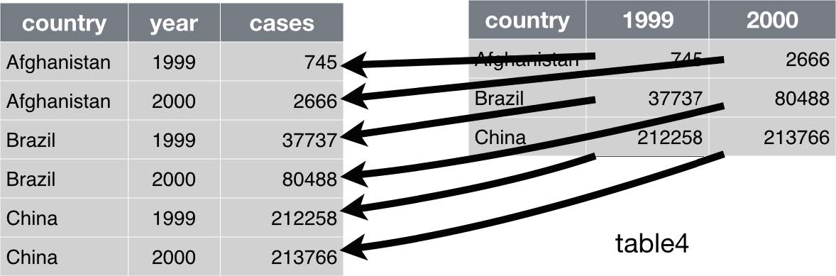
Recall table4a in the tidyverse package. This table is not tidy as the variable cases is scattered across two columns. In other words,

• The column names (1999 and 2000) should be values of the year variable
• The values (\(745, 2666, \cdots\)) should be values of the cases variable.

Example 1.1

table4a

library(tidyverse)
table4a
#> # A tibble: 3 × 3
#>   country     `1999` `2000`
#>   <chr>        <dbl>  <dbl>
#> 1 Afghanistan    745   2666
#> 2 Brazil       37737  80488
#> 3 China       212258 213766

Use pivot_longer() to “lengthen” the data table table4a

table4a %>% pivot_longer(cols = c(`1999`, `2000`), 
                         names_to = "year", 
                         values_to = "cases")
#> # A tibble: 6 × 3
#>   country     year   cases
#>   <chr>       <chr>  <dbl>
#> 1 Afghanistan 1999     745
#> 2 Afghanistan 2000    2666
#> 3 Brazil      1999   37737
#> 4 Brazil      2000   80488
#> 5 China       1999  212258
#> 6 China       2000  213766

Create table4 by join the tidy versions of table4a and table4b

• Use pivot_longer() to “lengthen” the data table table4a to table4a_tidy (variables: year and cases)
• Use pivot_longer() to “lengthen” the data table table4b to table4b_tidy (variables: year and population)
• Then join the two tidy tables to table4.

table4a_tidy <- table4a %>% pivot_longer(cols = c(`1999`, `2000`), 
                         names_to = "year", 
                         values_to = "cases")
table4b_tidy <- table4b %>% pivot_longer(cols = c(`1999`, `2000`), 
                         names_to = "year", 
                         values_to = "population")
table4 <- left_join(table4a_tidy, table4b_tidy)
table4
#> # A tibble: 6 × 4
#>   country     year   cases population
#>   <chr>       <chr>  <dbl>      <dbl>
#> 1 Afghanistan 1999     745   19987071
#> 2 Afghanistan 2000    2666   20595360
#> 3 Brazil      1999   37737  172006362
#> 4 Brazil      2000   80488  174504898
#> 5 China       1999  212258 1272915272
#> 6 China       2000  213766 1280428583

pivot_wider()

pivot_wider() – “widens” data, increasing the number of columns and decreasing the number of rows.

pivot_wider(data_frame, 
            names_from = name,
            values_from = value)

• names_from and values_from – a pair of arguments
• names_from – the original column where the new columns names are from
• values_from – the original column where the new columns values are from

Example 2

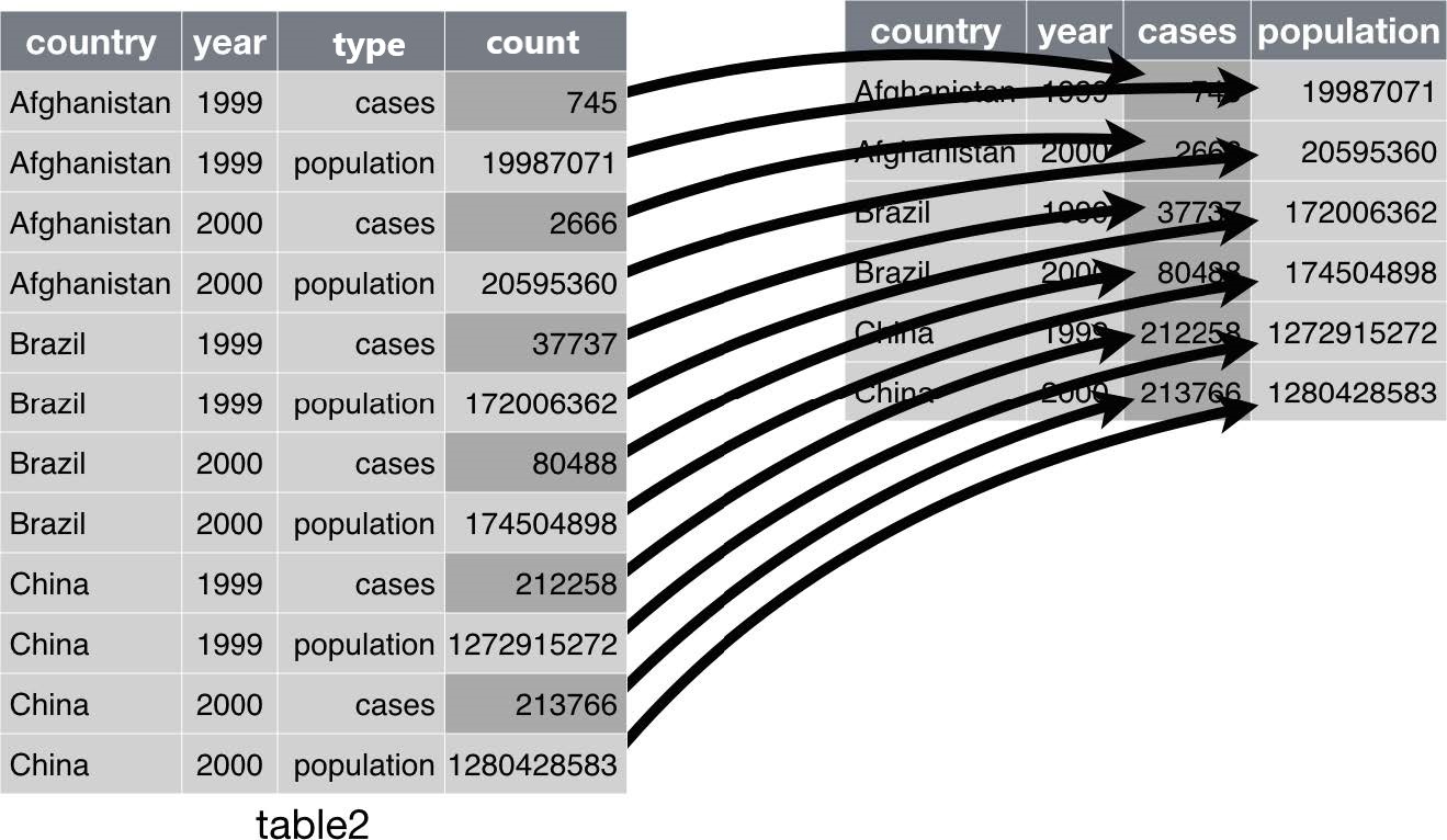
Recall table2. This table is not tidy as an observations is a country in a year, but each observation is spread across two rows. In other words,

• The cases and population should be variable names
• The values (\(745, 2666, \cdots\)) should be values of the cases or population variable.

Example 2.1

table2

table2
#> # A tibble: 12 × 4
#>    country      year type            count
#>    <chr>       <dbl> <chr>           <dbl>
#>  1 Afghanistan  1999 cases             745
#>  2 Afghanistan  1999 population   19987071
#>  3 Afghanistan  2000 cases            2666
#>  4 Afghanistan  2000 population   20595360
#>  5 Brazil       1999 cases           37737
#>  6 Brazil       1999 population  172006362
#>  7 Brazil       2000 cases           80488
#>  8 Brazil       2000 population  174504898
#>  9 China        1999 cases          212258
#> 10 China        1999 population 1272915272
#> 11 China        2000 cases          213766
#> 12 China        2000 population 1280428583

Use pivot_wider() to “widens” the data table table2

library(tidyverse)

table2 %>% pivot_wider(names_from = type, 
                       values_from = count)
#> # A tibble: 6 × 4
#>   country      year  cases population
#>   <chr>       <dbl>  <dbl>      <dbl>
#> 1 Afghanistan  1999    745   19987071
#> 2 Afghanistan  2000   2666   20595360
#> 3 Brazil       1999  37737  172006362
#> 4 Brazil       2000  80488  174504898
#> 5 China        1999 212258 1272915272
#> 6 China        2000 213766 1280428583

Separate

Turns a single character column into multiple columns:

• separate_wider_delim() – splits by delimiter
• separate_wider_position() – splits at fixed widths
• separate_wider_regex() – splits with regular expression matches

Example 3

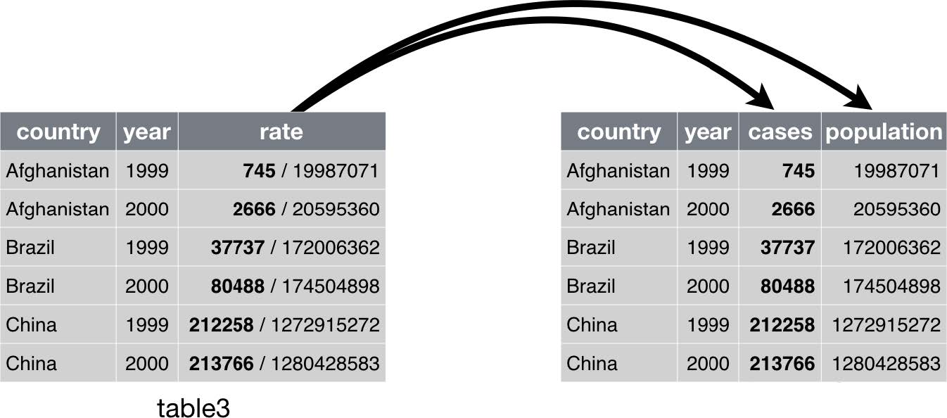
Recall table3. This table is not tidy as one column rate contains two variables cases and population. To fix this problem, we’ll need the separate-type functions.

table3 %>% 
  separate_wider_delim(rate, delim = "/", names =  c("cases", "population"))
#> # A tibble: 6 × 4
#>   country      year cases  population
#>   <chr>       <dbl> <chr>  <chr>     
#> 1 Afghanistan  1999 745    19987071  
#> 2 Afghanistan  2000 2666   20595360  
#> 3 Brazil       1999 37737  172006362 
#> 4 Brazil       2000 80488  174504898 
#> 5 China        1999 212258 1272915272
#> 6 China        2000 213766 1280428583

Using separate_wider_position() to separate the variable year in table3 to columns century (dropped) and year_last2.

table3 %>% 
  separate_wider_position(year, c(2, year_last2 = 2))
#> # A tibble: 6 × 3
#>   country     year_last2 rate             
#>   <chr>       <chr>      <chr>            
#> 1 Afghanistan 99         745/19987071     
#> 2 Afghanistan 00         2666/20595360    
#> 3 Brazil      99         37737/172006362  
#> 4 Brazil      00         80488/174504898  
#> 5 China       99         212258/1272915272
#> 6 China       00         213766/1280428583

unite()

unite() – a convenience function to paste together multiple columns into one.

unite(data_frame, 
      cols, 
      ### vector of columns to be combined
      sep)
      ### separator

Example 4

Combine the century and year values in table5.

table5
#> # A tibble: 6 × 4
#>   country     century year  rate             
#>   <chr>       <chr>   <chr> <chr>            
#> 1 Afghanistan 19      99    745/19987071     
#> 2 Afghanistan 20      00    2666/20595360    
#> 3 Brazil      19      99    37737/172006362  
#> 4 Brazil      20      00    80488/174504898  
#> 5 China       19      99    212258/1272915272
#> 6 China       20      00    213766/1280428583

unite() is the inverse of separate: it combines multiple columns into a single column.

We combine the century and year values.

table5 %>% 
  unite(new, century, year)
#> # A tibble: 6 × 3
#>   country     new   rate             
#>   <chr>       <chr> <chr>            
#> 1 Afghanistan 19_99 745/19987071     
#> 2 Afghanistan 20_00 2666/20595360    
#> 3 Brazil      19_99 37737/172006362  
#> 4 Brazil      20_00 80488/174504898  
#> 5 China       19_99 212258/1272915272
#> 6 China       20_00 213766/1280428583

• There is a understore between century and year above.
• Remove the underscore

table5 %>% 
  unite(new, century, year, sep = "")
#> # A tibble: 6 × 3
#>   country     new   rate             
#>   <chr>       <chr> <chr>            
#> 1 Afghanistan 1999  745/19987071     
#> 2 Afghanistan 2000  2666/20595360    
#> 3 Brazil      1999  37737/172006362  
#> 4 Brazil      2000  80488/174504898  
#> 5 China       1999  212258/1272915272
#> 6 China       2000  213766/1280428583

Understand joins

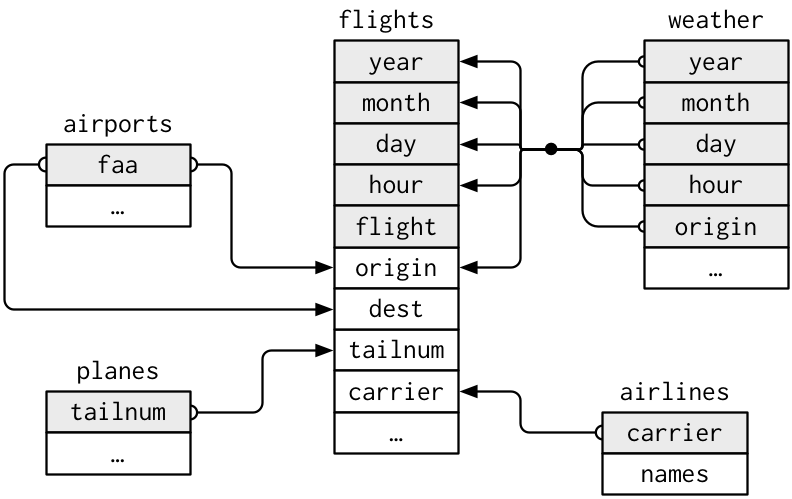
It’s rare that data analysis involves a single table of data. Multiple tables of data are called relational data.

For example, in the nycflights13 package, the airlines, airports, planes, weather are related to the flights data in the following way.

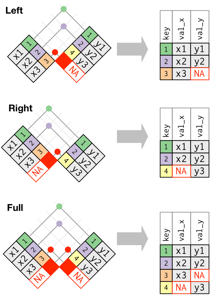
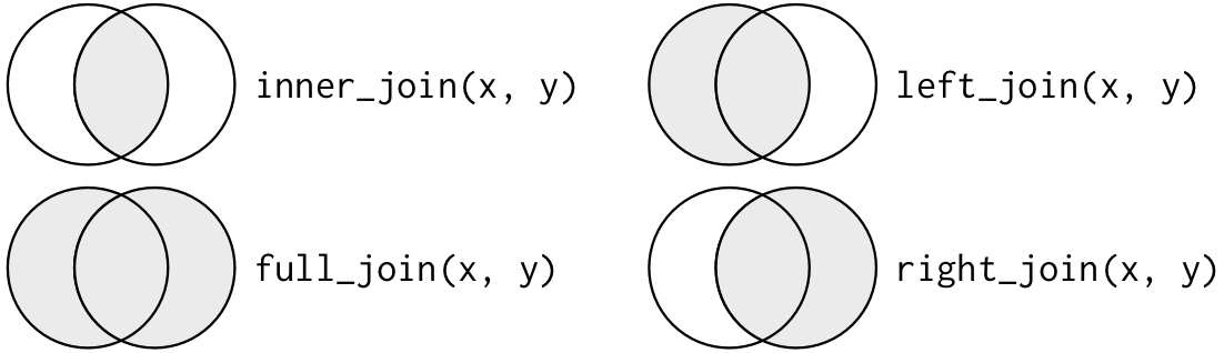
Different join functions

• inner_join()
• left_join()
• right_join()
• full_join()

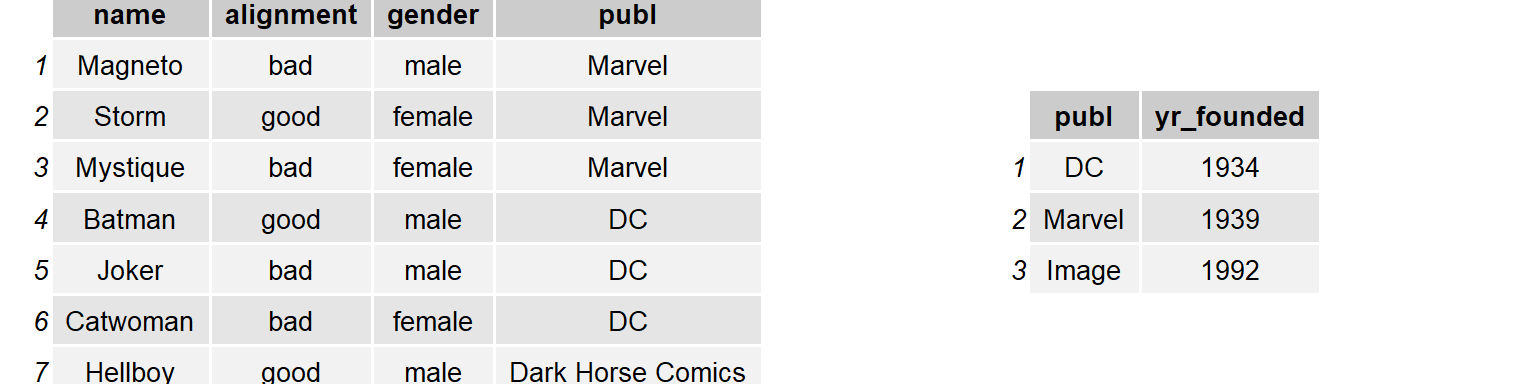
Example 5

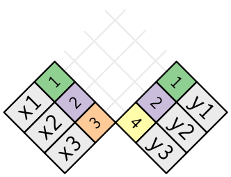
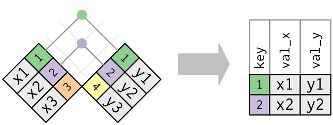
To learn how joins (left_join, right_join, inner_join, outer_join, etc.) works, we use the toy example and a visual representation below.

x <- tribble(
  ~key, ~val_x,
     1, "x1",
     2, "x2",
     3, "x3"
)
y <- tribble(
  ~key, ~val_y,
     1, "y1",
     2, "y2",
     4, "y3"
)

Inner join

x %>% inner_join(y, by = "key")
#> # A tibble: 2 × 3
#>     key val_x val_y
#>   <dbl> <chr> <chr>
#> 1     1 x1    y1   
#> 2     2 x2    y2

Outer joins

• left_join()
• right_join()
• full_join()

x %>% left_join(y, by = "key")
#> # A tibble: 3 × 3
#>     key val_x val_y
#>   <dbl> <chr> <chr>
#> 1     1 x1    y1   
#> 2     2 x2    y2   
#> 3     3 x3    <NA>
x %>% right_join(y, by = "key")
#> # A tibble: 3 × 3
#>     key val_x val_y
#>   <dbl> <chr> <chr>
#> 1     1 x1    y1   
#> 2     2 x2    y2   
#> 3     4 <NA>  y3
x %>% full_join(y, by = "key")
#> # A tibble: 4 × 3
#>     key val_x val_y
#>   <dbl> <chr> <chr>
#> 1     1 x1    y1   
#> 2     2 x2    y2   
#> 3     3 x3    <NA> 
#> 4     4 <NA>  y3

Another way to depict the different types of join is with a Venn diagram:

Example 6

Working with two small dataframes: superheroes and publishers.

superheroes <- tibble::tribble(
       ~name, ~alignment,  ~gender,          ~publ,
   "Magneto",      "bad",   "male",            "Marvel",
     "Storm",     "good", "female",            "Marvel",
  "Mystique",      "bad", "female",            "Marvel",
    "Batman",     "good",   "male",                "DC",
     "Joker",      "bad",   "male",                "DC",
  "Catwoman",      "bad", "female",                "DC",
   "Hellboy",     "good",   "male", "Dark Horse Comics"
  )

publishers <- tibble::tribble(
  ~publ, ~yr_founded,
        "DC",       1934L,
    "Marvel",       1939L,
     "Image",       1992L
  )

Let’s display the tibbles.

superheroes
#> # A tibble: 7 × 4
#>   name     alignment gender publ             
#>   <chr>    <chr>     <chr>  <chr>            
#> 1 Magneto  bad       male   Marvel           
#> 2 Storm    good      female Marvel           
#> 3 Mystique bad       female Marvel           
#> 4 Batman   good      male   DC               
#> 5 Joker    bad       male   DC               
#> 6 Catwoman bad       female DC               
#> 7 Hellboy  good      male   Dark Horse Comics

publishers
#> # A tibble: 3 × 2
#>   publ   yr_founded
#>   <chr>       <int>
#> 1 DC           1934
#> 2 Marvel       1939
#> 3 Image        1992

• The key variable name is publ, which needs to be exactly the same in the two dataframes.

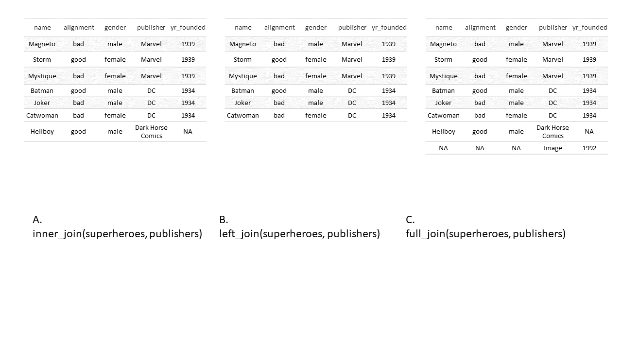
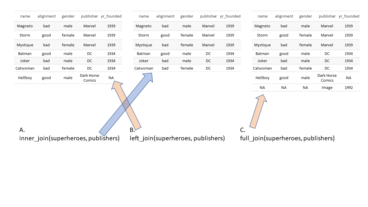
Quiz

• Tibbles superheroes and publishers

Please match the output tables with the join functions used.

Quiz Solution

• Tibbles superheroes and publishers

Please match the output tables with the join functions used.

Example 6.1 – inner_join()

superheroes %>% inner_join(publishers, by = "publ")
#> # A tibble: 6 × 5
#>   name     alignment gender publ   yr_founded
#>   <chr>    <chr>     <chr>  <chr>       <int>
#> 1 Magneto  bad       male   Marvel       1939
#> 2 Storm    good      female Marvel       1939
#> 3 Mystique bad       female Marvel       1939
#> 4 Batman   good      male   DC           1934
#> 5 Joker    bad       male   DC           1934
#> 6 Catwoman bad       female DC           1934

• inner_join returns all rows from superheros where there are matching values in publishers.
• We lose Hellboy as his publisher Dark Horse Comics does not appear in publishers.

Example 6.2 – left_join()

superheroes %>% left_join(publishers, by = "publ")
#> # A tibble: 7 × 5
#>   name     alignment gender publ              yr_founded
#>   <chr>    <chr>     <chr>  <chr>                  <int>
#> 1 Magneto  bad       male   Marvel                  1939
#> 2 Storm    good      female Marvel                  1939
#> 3 Mystique bad       female Marvel                  1939
#> 4 Batman   good      male   DC                      1934
#> 5 Joker    bad       male   DC                      1934
#> 6 Catwoman bad       female DC                      1934
#> 7 Hellboy  good      male   Dark Horse Comics         NA

• left_join returns all rows from superheros.
• We get all columns in superheros back, with the addition of variable yr_founded, which is unique to publishers.
• Hellboy, whose publisher Dark Horse Comics does not appear in publishers, has an NA for yr_founded.

Example 6.3 – right_join()

superheroes %>% right_join(publishers, by = "publ")
#> # A tibble: 7 × 5
#>   name     alignment gender publ   yr_founded
#>   <chr>    <chr>     <chr>  <chr>       <int>
#> 1 Magneto  bad       male   Marvel       1939
#> 2 Storm    good      female Marvel       1939
#> 3 Mystique bad       female Marvel       1939
#> 4 Batman   good      male   DC           1934
#> 5 Joker    bad       male   DC           1934
#> 6 Catwoman bad       female DC           1934
#> 7 <NA>     <NA>      <NA>   Image        1992

• right_join returns all rows from publishers.
• We get all columns in publishers back, with the addition of variables name, alignment, gender, which is unique to superheroes.
• Image, the publisher has no corresponding superhero, has NAs for name, alignment, gender.

Example 6.4 – full_join()

superheroes %>% full_join(publishers, by = "publ")
#> # A tibble: 8 × 5
#>   name     alignment gender publ              yr_founded
#>   <chr>    <chr>     <chr>  <chr>                  <int>
#> 1 Magneto  bad       male   Marvel                  1939
#> 2 Storm    good      female Marvel                  1939
#> 3 Mystique bad       female Marvel                  1939
#> 4 Batman   good      male   DC                      1934
#> 5 Joker    bad       male   DC                      1934
#> 6 Catwoman bad       female DC                      1934
#> 7 Hellboy  good      male   Dark Horse Comics         NA
#> 8 <NA>     <NA>      <NA>   Image                   1992

• rull_join returns all rows and columns from superheroes and publishers.
• Where there are not matching values, use NA.

Reference books

• R for Data Science: https://r4ds.hadley.nz/
• Hands-on Programming with R: https://rstudio-education.github.io/hopr/
• R Graphics Cookbook: https://r-graphics.org/
• Statistical Inference via Data Science: A Modern Dive into R and the Tidyverse, by Chester Ismay, Albert Y. Kim
• https://stat545.com/join-cheatsheet.html

Reference resources on tidyverse on github

https://github.com/stmorse/intro-tidyverse

https://github.com/rstudio-education/welcome-to-the-tidyverse