Data Manipulation with dplyr

dplyr

• Core member in tidyverse
• A package that transforms data
• dplyr implements a grammar for transforming tabular data.
• dplyr cheat sheet https://nyu-cdsc.github.io/learningr/assets/data-transformation.pdf

Commonly used commands in dplyr

• select() – extract variables
  • Recommended to always use dplyr::select()
• filter() – extract cases
• arrange() – reorder cases
• mutate() – create new variables
  • n() – number of values/rows
  • n_distinct() – number of unique
• group_by() – group cases
• summarize() – summarize variables
  • Note: summarise() and summarize() are synonyms.
  • Recommended to always use dplyr::summarize()
• count() – count number of rows in each group

select()

select() – Extract columns (variables) by name

• Select variables var1 and var3 from the data frame df

select(df, var1, var3)

• Select range of variables var1, var2, var3 from the data frame df

select(df, var1:var3)

• Select every column but variables var1 and var2 from the data frame df

select(df, -c(var1, var2))

• Select every column

select(df, everything())

select(df, var7, everything()) – Place var7 first, followed by all other variables

Example 1

Let’s use the mpg tibble in ggplot2. Please use help(mpg) for the variable definitions.

library(tidyverse)
mpg
#> # A tibble: 234 × 11
#>    manufacturer model      displ  year   cyl trans drv     cty   hwy fl    class
#>    <chr>        <chr>      <dbl> <int> <int> <chr> <chr> <int> <int> <chr> <chr>
#>  1 audi         a4           1.8  1999     4 auto… f        18    29 p     comp…
#>  2 audi         a4           1.8  1999     4 manu… f        21    29 p     comp…
#>  3 audi         a4           2    2008     4 manu… f        20    31 p     comp…
#>  4 audi         a4           2    2008     4 auto… f        21    30 p     comp…
#>  5 audi         a4           2.8  1999     6 auto… f        16    26 p     comp…
#>  6 audi         a4           2.8  1999     6 manu… f        18    26 p     comp…
#>  7 audi         a4           3.1  2008     6 auto… f        18    27 p     comp…
#>  8 audi         a4 quattro   1.8  1999     4 manu… 4        18    26 p     comp…
#>  9 audi         a4 quattro   1.8  1999     4 auto… 4        16    25 p     comp…
#> 10 audi         a4 quattro   2    2008     4 manu… 4        20    28 p     comp…
#> # ℹ 224 more rows

Recall: check missing values code chunk – from the previous lecture

mpg %>% 
  dplyr::select(everything()) %>% # use everything() to select all variables
  summarize_all(~sum(is.na(.))) # summarize_all() affects every variable
#> # A tibble: 1 × 11
#>   manufacturer model displ  year   cyl trans   drv   cty   hwy    fl class
#>          <int> <int> <int> <int> <int> <int> <int> <int> <int> <int> <int>
#> 1            0     0     0     0     0     0     0     0     0     0     0

Example 2

List the distinct model names (using the variable model) in the mpg tibble.

mpg %>% 
  dplyr::select(model) %>% 
  distinct()
#> # A tibble: 38 × 1
#>    model             
#>    <chr>             
#>  1 a4                
#>  2 a4 quattro        
#>  3 a6 quattro        
#>  4 c1500 suburban 2wd
#>  5 corvette          
#>  6 k1500 tahoe 4wd   
#>  7 malibu            
#>  8 caravan 2wd       
#>  9 dakota pickup 4wd 
#> 10 durango 4wd       
#> # ℹ 28 more rows

• There are 38 distinct model names!

Example 3

The model variable has too many categories to be useful. Please remove the column model and save the new tibble as mpg1.

mpg1 <- mpg %>% 
  dplyr::select(-model)
names(mpg1)
#>  [1] "manufacturer" "displ"        "year"         "cyl"          "trans"       
#>  [6] "drv"          "cty"          "hwy"          "fl"           "class"

filter()

filter() – Extract rows by logical criteria

Extract rows that meet logical criteria from the data frame df

filter(df, logical_criteria)

Logical Tests and Boolean Operators

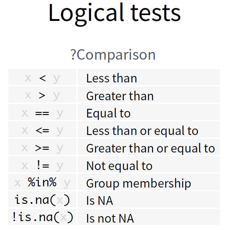
Example 4

From the mpg1 tibble, create a sub-tibble named DODGE with the manufacture being dodge only.

DODGE <- mpg1 %>% 
  filter(manufacturer == "dodge")
dim(DODGE)
#> [1] 37 10

Example 5

From the mpg1 tibble, create a sub-tibble named DODGE_SUV with the manufacture being dodge and vehicle class being suv.

DODGE_SUV <- mpg1 %>% 
  filter(manufacturer == "dodge" & class == 'suv')

# Or equivalently,
DODGE_SUV <- mpg1 %>% 
  filter(manufacturer == "dodge", class == 'suv')

dim(DODGE_SUV)
#> [1]  7 10

Example 6

Draw a scatterplot of hwy vs displ (highway mileage vs engine displacement in liters) for the Japanese cars only (the Japanese manufacturers are honda, nissan, subaru, or toyota), colored by manufacturer.

Example 6.1

From the mpg1 tibble, create a sub-tibble named Japanese_car.

Japanese_car <- mpg1 %>% filter(manufacturer %in% c("honda", "nissan", "subaru", "toyota"))
dim(Japanese_car)
#> [1] 70 10

Example 6.2

Use the Japanese_car tibble to draw the scatterplot of hwy vs displ. Recall that, geom_point() could be used.

ggplot(Japanese_car, aes(x = displ, y = hwy, col = manufacturer)) +
  geom_point()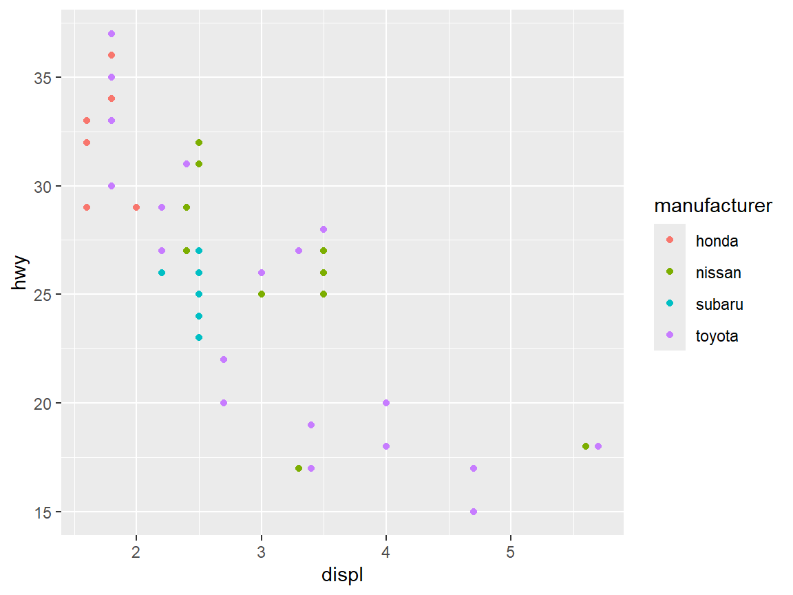

Combine the Example 6.1 and 6.2

mpg1 %>% 
  filter(manufacturer %in% c("honda", "nissan", "subaru", "toyota")) %>% 
  ggplot(aes(x=displ, y=hwy, col= manufacturer)) +
  geom_point()

arrange()

arrange() – reorder rows by the value of one or more columns (variables)

• arrange() is used to reorder rows of data.
• Order will be based on values in a specified column.
• The default order will be ascending order.
• To achieve descending order desc() will be used within arrange().

Example 7

In the workshop data (i.e. DS Workshop Participants List.csv), select the variables Name, Department, Major only, sort depend on the Major variable.

Step 1. Import the workshop data in csv into R, using read_csv() command in readr package.

tbl_workshop = read_csv("DS Workshop Participants List.csv")
tbl_workshop
#> # A tibble: 16 × 11
#>    Name       Gender `Email Address` Department `Info Source` `Class Year` Major
#>    <chr>      <chr>  <chr>           <chr>      <chr>         <chr>        <chr>
#>  1 Dwayne Jo… M      Djohnson@illin… Statistics Email         Undergradua… Stat…
#>  2 Rihanna    F      Rihanna@illino… Economics  Class         Graduate     ECON 
#>  3 Ellen DeG… F      Edegeneres@ill… Biology    Email         Undergradua… Biol…
#>  4 Will Smith M      Wsmith@illinoi… Electrica… Email         Undergradua… Elec…
#>  5 Angelina … F      Ajolie@illinoi… Computer … Class         Undergradua… Comp…
#>  6 Cristiano… M      Cronaldo@illin… Economics  Friends/Coll… Faculty and… <NA> 
#>  7 Leonardo … M      Ldicaprio@illi… Economics  Email         Undergradua… Econ…
#>  8 Tom Cruise M      Tcruise@illino… Mathemati… Class         Undergradua… Math…
#>  9 Robert Do… M      RDowneyJr@illi… mechanica… Class         Undergradua… Mech…
#> 10 Celine Di… F      Cdion@illinois… Biology    Friends/Coll… Faculty and… <NA> 
#> 11 Adele      F      Adele@illinois… Statistics Class         Undergradua… Stat…
#> 12 Serena Wi… F      Swilliams@illi… Computer … Email         Undergradua… Comp…
#> 13 Lionel Me… M      Lmessi@illinoi… Biology    Professor     Graduate     Biol…
#> 14 Taylor Sw… F      Tswift@illinoi… BIology    Flyer         Undergradua… Biol…
#> 15 J. K. Row… F      JKRowling@illi… Finance    Email         Undergradua… Fina…
#> 16 LeBron Ja… M      Ljames@illinoi… Electrica… Flyer         Undergradua… EE   
#> # ℹ 4 more variables: `Related Courses Taken` <chr>,
#> #   `Programming Language Known` <chr>,
#> #   `Willingness to be the Presenter` <chr>, `DS Years of Experience` <dbl>

Step 2. Select the columns Name, Department, Major only.

Step 3. Sort the tibble by Major.

tbl_workshop %>% 
  dplyr::select(Name, Department, Major) %>% 
  arrange(Major) 
#> # A tibble: 16 × 3
#>    Name              Department                          Major                 
#>    <chr>             <chr>                               <chr>                 
#>  1 Ellen DeGeneres   Biology                             Biology               
#>  2 Lionel Messi      Biology                             Biology               
#>  3 Taylor Swift      BIology                             Biology               
#>  4 Angelina Jolie    Computer Science                    Computer Science      
#>  5 Serena Williams   Computer Science                    Computer Science      
#>  6 Rihanna           Economics                           ECON                  
#>  7 LeBron James      Electrical and Computer Engineering EE                    
#>  8 Leonardo DiCaprio Economics                           Economics             
#>  9 Will Smith        Electrical and Computer Engineering Electrical Engineering
#> 10 J. K. Rowling     Finance                             Finance               
#> 11 Tom Cruise        Mathematics                         Mathematics           
#> 12 Robert Downey Jr. mechanical Science and Engineering  Mechanical Engineering
#> 13 Dwayne Johnson    Statistics                          Statistics            
#> 14 Adele             Statistics                          Statistics            
#> 15 Cristiano Ronaldo Economics                           <NA>                  
#> 16 Celine Dion       Biology                             <NA>

Note that:

• The tibble is sorted by Major in alphabetical order, in ascending order.

• Missing values (i.e. NA) are always sorted at the end.

Example 7 (continue)

In the workshop data (i.e. DS Workshop Participants List.csv), select the variables Name, Department, Major only, sort depend on the Major variable.

If sort the tibble by Major in descending order is preferred…

tbl_workshop %>% 
  dplyr::select(Name, Department, Major) %>% 
  arrange(desc(Major)) ### Use desc() to re-order in descending order
#> # A tibble: 16 × 3
#>    Name              Department                          Major                 
#>    <chr>             <chr>                               <chr>                 
#>  1 Dwayne Johnson    Statistics                          Statistics            
#>  2 Adele             Statistics                          Statistics            
#>  3 Robert Downey Jr. mechanical Science and Engineering  Mechanical Engineering
#>  4 Tom Cruise        Mathematics                         Mathematics           
#>  5 J. K. Rowling     Finance                             Finance               
#>  6 Will Smith        Electrical and Computer Engineering Electrical Engineering
#>  7 Leonardo DiCaprio Economics                           Economics             
#>  8 LeBron James      Electrical and Computer Engineering EE                    
#>  9 Rihanna           Economics                           ECON                  
#> 10 Angelina Jolie    Computer Science                    Computer Science      
#> 11 Serena Williams   Computer Science                    Computer Science      
#> 12 Ellen DeGeneres   Biology                             Biology               
#> 13 Lionel Messi      Biology                             Biology               
#> 14 Taylor Swift      BIology                             Biology               
#> 15 Cristiano Ronaldo Economics                           <NA>                  
#> 16 Celine Dion       Biology                             <NA>

Example 8

From the mpg1 tibble, draw a bar graph of the vehicle classes (variable class) to go in descending order.

Example 8.1

Draw a bar graph of vehicle classes.

ggplot(mpg1, aes(class)) +
  geom_bar() 

Example 8

From the mpg1 tibble, draw a bar graph of the vehicle classes (variable class) to go in descending order.

Example 8.2

Use arrange() to sort the bar graph in descending order.

Step 1. Find the counts for each class type

mpg1 %>% count(class)
#> # A tibble: 7 × 2
#>   class          n
#>   <chr>      <int>
#> 1 2seater        5
#> 2 compact       47
#> 3 midsize       41
#> 4 minivan       11
#> 5 pickup        33
#> 6 subcompact    35
#> 7 suv           62

Step 2. Use arrange() to sort the counts

mpg1 %>% count(class) %>% 
  arrange(desc(n)) ## desc() means in descending order
#> # A tibble: 7 × 2
#>   class          n
#>   <chr>      <int>
#> 1 suv           62
#> 2 compact       47
#> 3 midsize       41
#> 4 subcompact    35
#> 5 pickup        33
#> 6 minivan       11
#> 7 2seater        5

Step 3. Chain the code to ggplot with geom_col()

mpg1 %>% count(class) %>% 
  arrange(desc(n)) %>%
  ggplot(aes(class, n))+
  geom_col()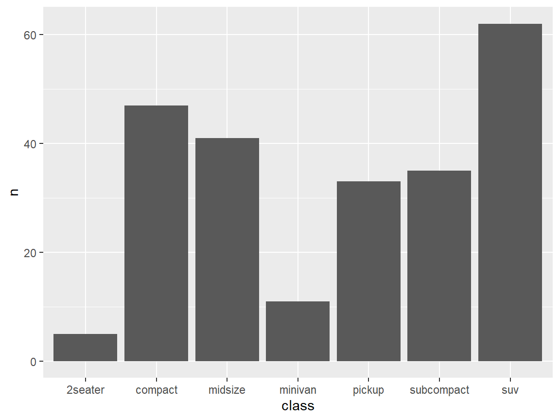 

Q: arrange() has been used. Why still not sorted?

Example 8

Draw a bar graph of the vehicle classes (variable class) to go in descending order.

Example 8.2 (continue)

Q: arrange() has been used. Why the bar graph created is still not sorted?

A: You need to save the order.

Code from the previous slide

mpg1 %>% count(class) %>%
  arrange(desc(n)) %>%
  ggplot(aes(class, n))+
  geom_col() 

Output after using arrange()

mpg1 %>% count(class) %>%
  arrange(desc(n))
#> # A tibble: 7 × 2
#>   class          n
#>   <chr>      <int>
#> 1 suv           62
#> 2 compact       47
#> 3 midsize       41
#> 4 subcompact    35
#> 5 pickup        33
#> 6 minivan       11
#> 7 2seater        5

Then use fct_inorder() to keep this descending order.

• fct_inorder() – Reorder factor levels by the order in which they first appear.

mpg1 %>% count(class) %>%
  arrange(desc(n)) %>%
  mutate(class = fct_inorder(class))%>% ### save the order
  ggplot(aes(class, n))+
  geom_col()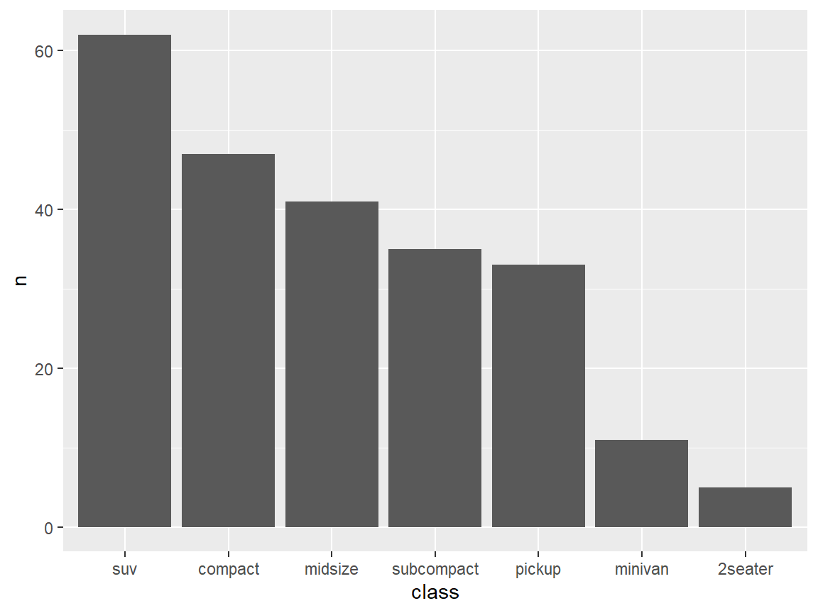

Example 9. Sort the data by multiple variables

From the mpg1 tibble, create a tibble that satisfies:

1. the manufacture is toyota,
2. select variables class, year, displ only,
3. sort the tibble depend on class, year, and displ, where class and year are in ascending order, displ is in descending order.

mpg1 %>% filter(manufacturer == "toyota") %>% 
  dplyr::select(class, year, displ) %>% 
  arrange(class, year, desc(displ)) %>% 
  print(n=15) ### Print 15 rows
#> # A tibble: 34 × 3
#>    class    year displ
#>    <chr>   <int> <dbl>
#>  1 compact  1999   3  
#>  2 compact  1999   3  
#>  3 compact  1999   2.2
#>  4 compact  1999   2.2
#>  5 compact  1999   1.8
#>  6 compact  1999   1.8
#>  7 compact  1999   1.8
#>  8 compact  2008   3.3
#>  9 compact  2008   2.4
#> 10 compact  2008   2.4
#> 11 compact  2008   1.8
#> 12 compact  2008   1.8
#> 13 midsize  1999   3  
#> 14 midsize  1999   3  
#> 15 midsize  1999   2.2
#> # ℹ 19 more rows

From the output above, it seems like the displ values increase as the year grow for the compact vehicle type. Is it true for the other vehicle types?

We could create a scatterplot to visualize the change.

mpg %>% filter(manufacturer == "toyota") %>% 
  dplyr::select(class, year, displ) %>% 
  ggplot(aes(x = year, y = displ))+
  geom_jitter(size = 3, height = 0, width = 0.3, alpha = 0.5)+
  geom_smooth(se = FALSE) +
  facet_wrap(~class)

–>

mutate()

• Use mutate() to add new variables and preserves existing ones.

Example 10

Please create a new column combined_mpg in mpg using the formula of

combined_mpg = 0.55 * cty + 0.45 * hwy

mpg %>% mutate(combined_mpg = 0.55*cty + 0.45*hwy) %>% 
  print(width = Inf) ## use print(width = Inf) to display all the columns
#> # A tibble: 234 × 12
#>    manufacturer model      displ  year   cyl trans      drv     cty   hwy fl   
#>    <chr>        <chr>      <dbl> <int> <int> <chr>      <chr> <int> <int> <chr>
#>  1 audi         a4           1.8  1999     4 auto(l5)   f        18    29 p    
#>  2 audi         a4           1.8  1999     4 manual(m5) f        21    29 p    
#>  3 audi         a4           2    2008     4 manual(m6) f        20    31 p    
#>  4 audi         a4           2    2008     4 auto(av)   f        21    30 p    
#>  5 audi         a4           2.8  1999     6 auto(l5)   f        16    26 p    
#>  6 audi         a4           2.8  1999     6 manual(m5) f        18    26 p    
#>  7 audi         a4           3.1  2008     6 auto(av)   f        18    27 p    
#>  8 audi         a4 quattro   1.8  1999     4 manual(m5) 4        18    26 p    
#>  9 audi         a4 quattro   1.8  1999     4 auto(l5)   4        16    25 p    
#> 10 audi         a4 quattro   2    2008     4 manual(m6) 4        20    28 p    
#>    class   combined_mpg
#>    <chr>          <dbl>
#>  1 compact         23.0
#>  2 compact         24.6
#>  3 compact         25.0
#>  4 compact         25.0
#>  5 compact         20.5
#>  6 compact         21.6
#>  7 compact         22.0
#>  8 compact         21.6
#>  9 compact         20.0
#> 10 compact         23.6
#> # ℹ 224 more rows

Example 11

Please compare the frequency and engine displacement average (variable displ) between the two transmissions (auto vs manual).

Example 11.1

Let’s first find the distinct transmission types (with sub types).

• Use distinct() to display the distinct transmission types (with sub types) – variable trans.

• Use n_distinct to find how many transmission types (with sub types).

Example 11

Please compare the frequency and engine displacement average (variable displ) between the two transmissions (auto vs manual).

Example 11.1

Let’s first find the distinct transmission types with sub types.

• Use distinct() to display the distinct transmission types (with sub types) – variable trans.

• Use n_distinct to find how many transmission types (with sub types).

mpg %>% 
  select(trans) %>%
  distinct()
#> # A tibble: 10 × 1
#>    trans     
#>    <chr>     
#>  1 auto(l5)  
#>  2 manual(m5)
#>  3 manual(m6)
#>  4 auto(av)  
#>  5 auto(s6)  
#>  6 auto(l4)  
#>  7 auto(l3)  
#>  8 auto(l6)  
#>  9 auto(s5)  
#> 10 auto(s4)

### Find just the count of distinct categories
mpg %>% 
  select(trans) %>%
  n_distinct()
#> [1] 10

• There are 10 distinct transmission types with sub types.
• But we only need to compare auto and manual transmission types.

Example 11

Please compare the frequency and engine displacement average (variable displ) between the two transmissions (auto vs manual).

Example 11.2

Use mutate() function to create a new variable trans with transmission type only, without sub types.

Example 11

Please compare the frequency and engine displacement average (variable displ) between the two transmissions (auto vs manual).

Example 11.2

Use mutate() function to create a new variable trans_type with transmission type only, without sub types.

mpg_transtype <- mpg %>%
  rowwise() %>% ## rowwise() groups the data by row. 
  mutate(trans_type = str_split(trans, "\\(")[[1]][1]) %>%
  ungroup() ## Use ungroup() to drop the rowwise behavior. 

mpg_transtype %>% distinct(trans_type)
#> # A tibble: 2 × 1
#>   trans_type
#>   <chr>     
#> 1 auto      
#> 2 manual

Do you have questions about the code above?

Please find the illustration in the next two slides of

• str_split(trans, "\\(")[[1]][1]
• rowwise()

Example 11.2 code – illustration of str_split()

• str_split() is from stringr package. The function can be used to split a string into multiple pieces.

str_split(string, pattern)

where

* string is a character vector,
* pattern is the pattern to split on.

• In this example,
  • you type \\( to match (, which is the separator.

  

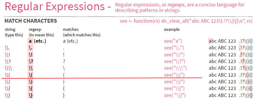
  • Please refer to the stringr cheat sheet for more information.

str_split("auto(l5)", "\\(")
#> [[1]]
#> [1] "auto" "l5)"

• We only need “auto” in this example. Therefore,

  • Use [[1]] to get the first element in this list – result in a vector,
  • Then use [1] get the first value of the vector.

str_split("auto(l5)", "\\(")[[1]]
#> [1] "auto" "l5)"

str_split("auto(l5)", "\\(")[[1]][1]
#> [1] "auto"

Example 11.2 code – illustration of rowwise()

If rowwise() is not used,

mpg %>% 
  mutate(trans_type = str_split(trans, "\\(")[[1]][1]) %>% 
  dplyr::select(trans_type, trans)
#> # A tibble: 234 × 2
#>    trans_type trans     
#>    <chr>      <chr>     
#>  1 auto       auto(l5)  
#>  2 auto       manual(m5)
#>  3 auto       manual(m6)
#>  4 auto       auto(av)  
#>  5 auto       auto(l5)  
#>  6 auto       manual(m5)
#>  7 auto       auto(av)  
#>  8 auto       manual(m5)
#>  9 auto       auto(l5)  
#> 10 auto       manual(m6)
#> # ℹ 224 more rows

All are `auto’s in the trans column!

• Therefore, we need to perform the calculation by row to get the values for variable trans.
• After the mutate() function, use ungroup() to drop the rowwise behavior.

group_by(), summarize(), count()

Summarize information by groups

• Find summary statistics by group

• Useful function

  • Center: mean(), median()
  • Spread: sd(), IQR(), mad()
  • Range: min(), max(), quantile()
  • Position: first(), last(), nth()
  • Count: n(), n_distinct()
  • Logical: any(), all()

Example 11

Please compare the frequency and engine displacement average (variable displ) between the two transmissions (auto vs manual).

Example 11.3

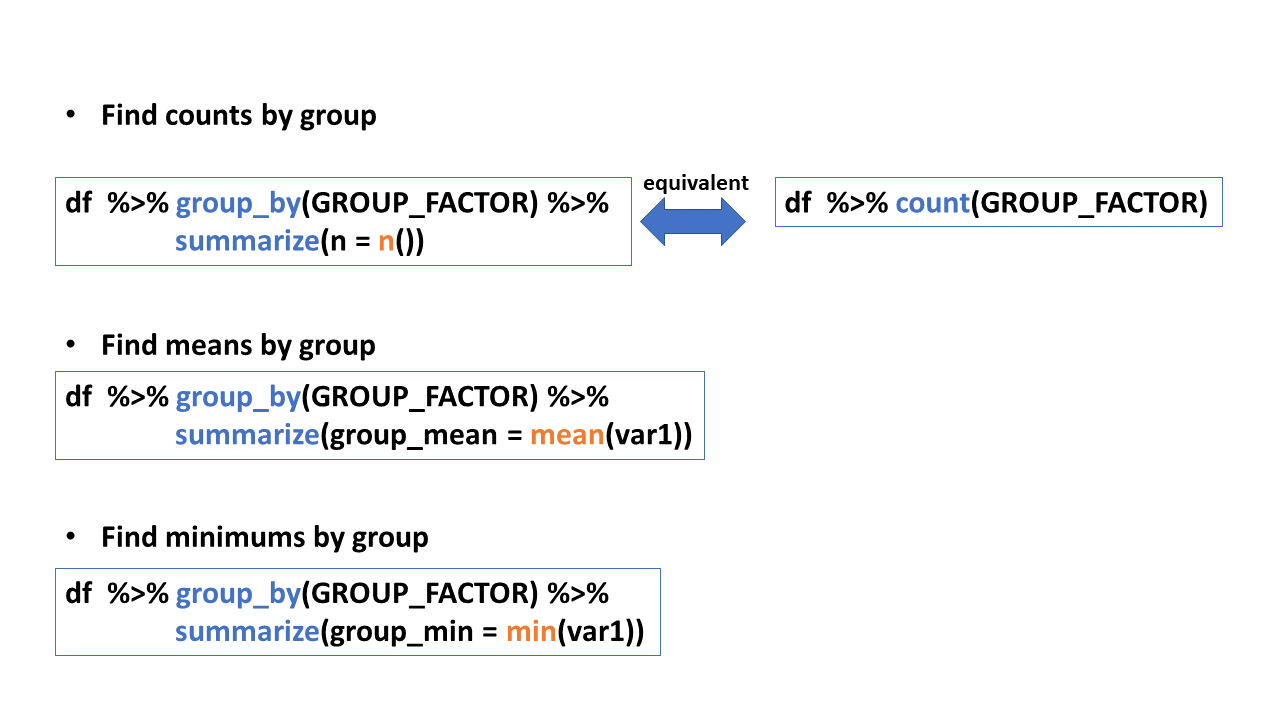
Use group_by(), summarize() and n() to find the frequency of the two transmission types.

Frequency table

mpg_transtype %>% 
  group_by(trans_type) %>%
  dplyr::summarize(freq = n())
#> # A tibble: 2 × 2
#>   trans_type  freq
#>   <chr>      <int>
#> 1 auto         157
#> 2 manual        77

### Or equivalently,
mpg_transtype %>% count(trans_type)
#> # A tibble: 2 × 2
#>   trans_type     n
#>   <chr>      <int>
#> 1 auto         157
#> 2 manual        77

Bar graph

We could show the counts visually using ggplot.

mpg_transtype %>% 
  group_by(trans_type) %>%
  dplyr::summarize(freq = n()) %>%
  ggplot(aes(trans_type, freq)) +
  geom_col()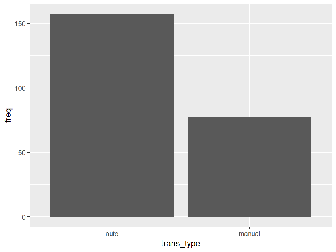

Example 11

Please compare the frequency and engine displacement average (variable displ) between the two transmissions (auto vs manual).

Example 11.4

Use mean() to compare the engine displacement average between the two transmissions (auto, manual).

mpg_transtype %>% 
  group_by(trans_type) %>%
  dplyr::summarize(displ_avg = mean(displ))
#> # A tibble: 2 × 2
#>   trans_type displ_avg
#>   <chr>          <dbl>
#> 1 auto            3.72
#> 2 manual          2.97

### or Visually using ggplot
mpg_transtype %>% 
  group_by(trans_type) %>%
  dplyr::summarize(displ_avg = mean(displ)) %>%
  ggplot(aes(trans_type, displ_avg))+
  geom_col()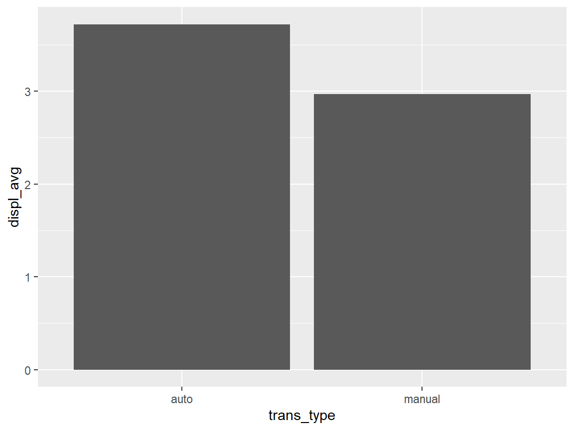

Example 11.5

If you need to

• group by multiple variables, or
• calculate several grouped summary statistics

Please read Example 11.5 on the next slide.

Example 11.5

Get a list of grouped summary statistics (min, Q1, median, Q3, max, mean, std. dev., missing) by transmission type (without sub group) and class type.

displ_summary <- mpg_transtype %>%
  group_by(trans_type, class)%>%
  dplyr::summarize(
    min = min(displ, na.rm = TRUE),
    q1 = quantile(displ, 0.25, na.rm = TRUE),
    median = quantile(displ, 0.5, na.rm = TRUE),
    q3 = quantile(displ, 0.75, na.rm = TRUE),
    max = max(displ, na.rm = TRUE),
    mean = mean(displ, na.rm = TRUE),
    sd = sd(displ, na.rm = TRUE),
    missing = sum(is.na(displ))
  )

displ_summary
#> # A tibble: 13 × 10
#> # Groups:   trans_type [2]
#>    trans_type class        min    q1 median    q3   max  mean    sd missing
#>    <chr>      <chr>      <dbl> <dbl>  <dbl> <dbl> <dbl> <dbl> <dbl>   <int>
#>  1 auto       2seater      5.7  5.82   5.95  6.08   6.2  5.95 0.354       0
#>  2 auto       compact      1.8  2      2.3   2.8    3.3  2.35 0.485       0
#>  3 auto       midsize      1.8  2.4    3.1   3.5    5.3  3.08 0.750       0
#>  4 auto       minivan      2.4  3.3    3.3   3.8    4    3.39 0.453       0
#>  5 auto       pickup       2.7  4.15   4.7   5.2    5.9  4.61 0.789       0
#>  6 auto       subcompact   1.6  1.87   2.1   2.98   4.6  2.6  1.05        0
#>  7 auto       suv          2.5  4      4.7   5.4    6.5  4.64 0.964       0
#>  8 manual     2seater      5.7  5.95   6.2   6.6    7    6.3  0.656       0
#>  9 manual     compact      1.8  2      2.2   2.65   3.1  2.3  0.425       0
#> 10 manual     midsize      1.8  2.35   2.45  2.85   3.5  2.54 0.470       0
#> 11 manual     pickup       2.7  3.7    4.2   4.7    5.2  4.13 0.835       0
#> 12 manual     subcompact   1.6  1.95   2.2   3.25   5.4  2.71 1.17        0
#> 13 manual     suv          2.5  2.5    2.7   3.35   4    2.99 0.590       0